In part one I demonstrated how we can use gene annotations to quickly generate synteny plots using MCscan. Here, we’ll narrow in a bit and generate synteny plots for fine-grain structural changes using Syri and genome alignments. Thumbnail from: https://github.com/schneebergerlab/syri

Introduction

In the previous post, I explored using MCscan to generate whole chromosome synteny plots, using gene annotations as anchors to find syntenic regions between chromosomes. MCscan works great if you have an annotation file, or are able to generate a rough annotation file if your organism doesn’t have one. The reason we explored using it is for a couple of reasons.

1. It’s simple to use, providing wrapper functions for many of the tedious tasks that would normally be involved in such an analysis
2. Using gene sequences as anchors for alignments makes it fast. Especially compared to traditional sequence alignment tools
3. It has built in helper functions to generate publication ready figures

However, if you don’t have gene annotaitons, or can’t generate rough ones easily, MCscan is no longer an option. Further, MCscan is great for macro-scale comparisons, but is not the best choice if you are interested in micro-synteny. Here, we’ll dive into using the tool Syri to generate micro-synteny plots that rely only on sequence alignment.

The software and data

For this analysis, we’re going to need a few tools to get the job done. The first is a sequence aligner that can handle whole genome alignments. There are many tools that are capable of this, however we’re going to use Minimap2. This is a fast alignment tool that can many sequence types including, short-read DNA/RNA, third generation sequences (Nanopore/PacBio) and whole genome alignments of varying divergence. We’re going to use Minimap2 as it is fast, simple to use and generates easy to use alignment files (SAM). The next tool we’ll need is Syri, which compares alignments bewteen two sequences, identifying synteny and structural rearrangements. Lastly, we’ll need the tool plotsr, which is used to generate the final figures. A summary of what each tool is used for is below:

• Minimap2: Align chromosomal sequences
• Syri: Identify sytenic regions/rearrangements between the aligned chromosomes
• Plotsr: Generate publication ready plots from the Syri output

We’re going to install this software using conda. I recommend installing Minimap2 into an environment of its own, and Syri and plotsr into a different environment together. This could be done as follows.

conda create -n minimap2 -c bioconda minimap2
conda create -n synteny -c bioconda syri plotsr

These two commands will create the environments minimap2 which houses the Minimap2 software and synteny which contains the Syri and plotsr software. Once created, the environments can be activated using the following command.

conda activate <env name here>

The sequences we’re going to align are provided in the Box directory Syri-resources/seqs directory. These sequences are the first 5Mbp of chromosome 1 from Hydrophis major and Hydrophis cyanocinctus. In there, you’ll also find some gene annotations for H. major (seqs/hydmaj.gff3) which we’ll use for plotting later on.

While I’ll provide relevant code here in the tutorial, I have written a script that has all the steps that can be found in synteny-resources/script/syri-tutorial.sh. Please note that you’ll need to change the paths to directories and files to match your own system!

Step 1: Minimap2 alignment of chromosomal sequences

Create chromosome sequence subsets

We first need to align the chromosomal sequences for H. major and H. cyanocinctus. Noramlly, we’d align all the chromosomes from one species against all the chromosomes of the other. For the sake of time, we’re going to use a smaller 5Mbp subset of the start of chromosome 1. For interests sake, 5Mbp subset files were generated using the following code.

samtools faidx assembly.fa chr1 > assembly-subset.fa

Align the sequences using Minimap2

To align the sequences we need to call Minimap2. The command recommended by the Syri developers is as follows.

conda activate minimap2
minimap2 \
    -ax asm5 \
    --eqx \
    -t threads \
    hydmaj-subset.fa \
    hydcya-subset.fa > hydmaj-hydcya.sam
conda deactivate

In the command above we provide the argument -a to specify we want SAM output rather than PAF. We also provide the -x asm5 argument to specify the assembly-to-assembly alignment preset with 0.1% sequence divergence. The argument --eqx is to output =/X CIGAR operators in the SAM file (information about mismatches) while the -t argument specifies how many threads we’ll want to use. The output from this command is the alignment between the two 5Mbp sequences which is stored in the file hydmaj-hydcya.sam.

Important to note is the activation and deactivation of the conda environment before running the program.

Optional: Convert the alignment file to BAM format

I have not done it here, but you can also convert the SAM file to BAM format if you want to save some space. As we’re only aligning a few megabases of sequences, the SAM file doesn’t get too large. However, if you’re doing this on whole genomes, it would be prudent to convert the output to BAM format before continuing. This could be managed as follows.

conda activate minimap2
minimap2 \
    -ax asm5 \
    --eqx \
    -t threads \
    hydmaj-subset.fa \
    hydcya-subset.fa |
samtools view -b -o hydmaj-hydcya.bam
conda deactivate

The example above pipes the output from Minimap2 to SAMtools to conver the SAM output to BAM format, by specifying the -b argument. This example assumes that samtools is installed in the minimap2 conda environment.

Step 2: Syri to find synteny/rearrangements

Now that we’ve got our alignment sorted, we can use Syri to find syntenic regions and structural rearrangements. All we need to do is run the software like so.

conda activate syri
syri \
    -c hydmaj-hydcya.sam \
    -r hydmaj-subset.fa \
    -q hydcya-subset.fa \
    -F S \
    --cigar
conda deactivate

The command above takes as input the SAM alignment file we generated (-c) along with each of the sequences of interest, with -r being the reference sequences and q being the query. What this means is that the query sequence will be compared to the reference.

This is an important point about Syri: it is not reference free. This means that all comparisons will always be ‘in reference’ to some particular sequence. This is good if we only want to compare between a few organisms, as we can simply run a hierarchy of comparisons e.g. A - B and B - C. This would enable us to see how A compares to B, which is in turn compared to organism C. As the number of species increases, it is perhaps better to use reference free tools like Progressive Cactus or Pan-Genome Graph Builder, which allows us to compare all sequences at once without requiring one organisms being designated the anchor reference to which all other organisms are aligned.

Back to our Syri command. After providing the two sequences we aligned, we next provide the file format (-F S for SAM)a along with the argument --cigar. This argument is required if we want to find SNP/INDELs using SAM/BAM alignment files.

This process will output the file syri.out in the directory where the command is run, so keep that in mind if you run this yourself. For information about the output format, see the documentation here.

Step 3: Generate synteny plots

The final step is to plot the information in the syri.out file. The same group that wrote Syri wrote the plotting tool plotsr. Below I’ll walk through generating a simple synteny plot, the introduce a few steps we can take to zhoosh it up a bit. Before we do anything though, we need to create a genomes.txt file.

Genomes file

The genome.txt file provides a bit of -data about the genomes we’ve compared. It is a tab-separated, three-columned file, with the three columns being 1) the path to the file, 2) the organisms name and 3) tags.. For our data, the file looks like so, which can be found in the syri output directory on Box.

/path/to/seqs/hydmaj-subset.fa	Hydrophis major	lw:1.5
/path/to/seqs/hydcya-subset.fa	Hydriophis cyanocinctus	lw:1.5

To create this file, copy the text above (ensureing the tab-spacing is maintained) into a file called genomes.txt in the syri output directory (where the SAM alignment file is stored).

Basic synteny plot

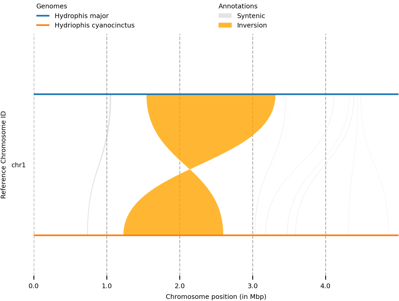
To generate a basic synteny plot using out output, we can simply run the following command.

plotsr \
     --sr syri.out \
     -o basic.png \
     --genomes genomes.txt \
     -W 6 \
     -H 4

This simply plots the information in syri.out, using the genome information from the genomes.txt file. The file is then saved to basic.png in the current directory and look like the following image.

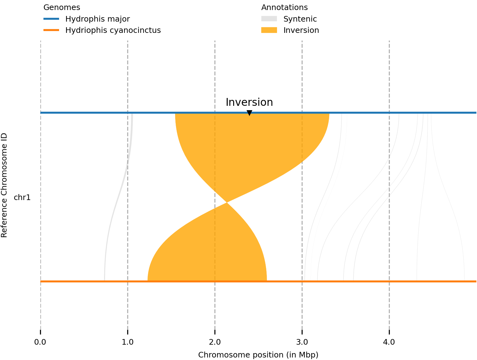
Adding markers

The image above conveys a lot of information in the legend, but perhaps we’d like to annotate the features on the tracks themselves. This can be done by creating and passing a markers.bed file to plotsr. This is a simple BED file with coordinate information about where to put markers. The developers have put together a list of the types of markers you can use in your plot here. I’ve put together an example markers.bed file in the syri output directory.

#chr	start	end genome_id	tags
chr1	2400000	2400001	Hydrophis major	mt:v;mc:black;ms:3;tt:Inversion;tp:0.02;ts:8;tf:DejaVu Sans;tc:black

To use the marker information in the plot, we simply need to add the --markers argument to our call.

plotsr \
     --sr syri.out \
     -o markers.png \
     --genomes genomes.txt \
     --markers markers.bed \
     -W 6 \
     -H 4

In the plot below, you can see we now have ‘inversion’ marked on the track itself. This example is pretty basic, but could be used to highlight key features in the figure.

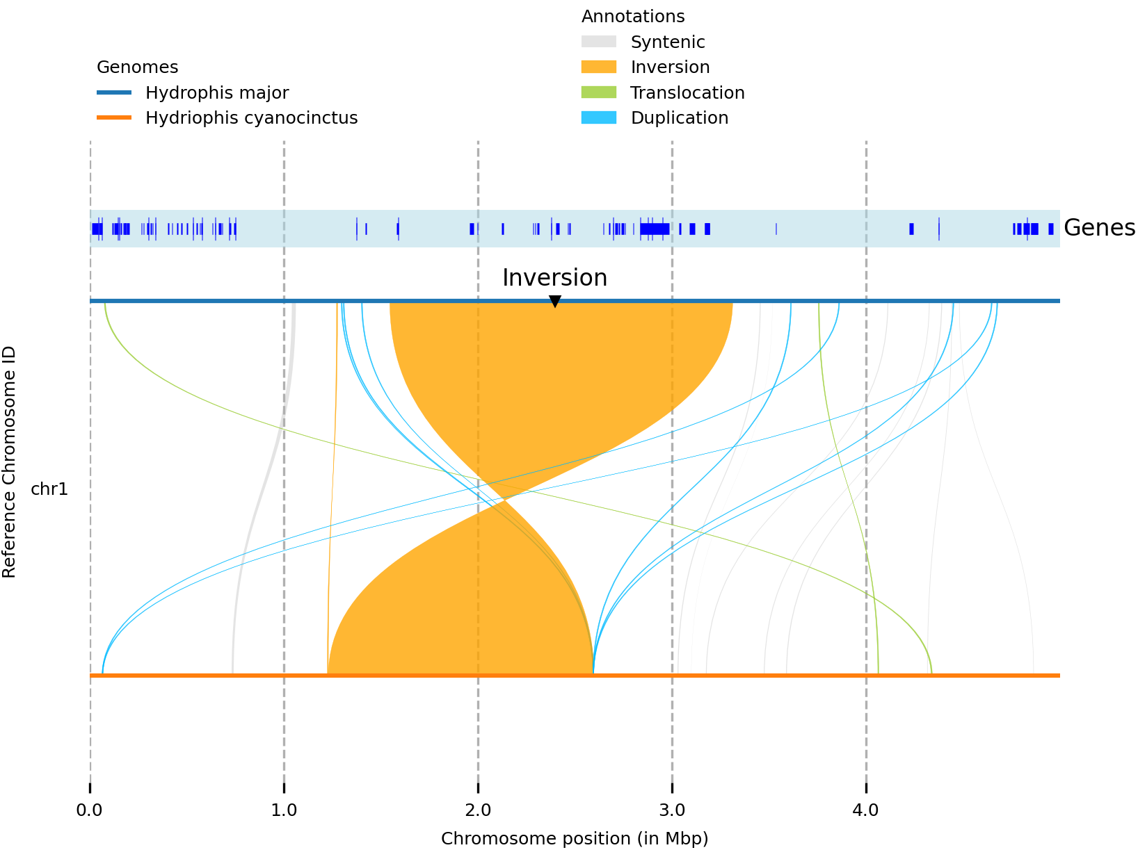
Adding tracks

The final thing we might like to do is overlay a track of some kind. The tracks.txt file houses information about genetic feature files that we want to overlay on the figure. Genetic features are usually stored in BED or GFF files, which represent the coordinates of genetic features we want to present/overlay. The tracks.txt file has three columns: 1) the path to the feature file 2) the name of the track and 3) tags associated with that feature track.

I’ve provided an example tracks.txt in the syri directory which points to the gene annotaitons for chromosome 1 of H. major. Importantly, the tracks that we want to overlay must correspond to the first genome (i.e. the reference sequence) in the alignment. In our case this is H. major. The example looks like the following.

# File	Name	Tags
/path/to/seqs/hydmaj.gff3	Genes	ft:gff;nc:black;ns:8;nf:DejaVu Sans;lc:blue;lw:4;bc:lightblue;ba:0.5

Again, to include the track information, we simply add the --tracks argument to our plotsr call (I also changed the minimum size for structural rearrangements to 5000bp in this example too: -s 5000).

plotsr \
     --sr syri.out \
     -o tracks.png \
     --genomes genomes.txt \
     --markers markers.bed \
     --tracks tracks.txt \
     -s 5000 \
     -W 6 \
     -H 4

The output of which looks like this

What next?

This document provides an introduction to the tools needed to generate micro-synteny plots. There are many other parameters that can be tweaked to get the sequences and plots just how you want them, so I encourage you to mess around with the commands until you get what you’re after.

A lot of the material I’ve put in here has come from the github repositories/documentation written by the devs. I highly recommend you go and check these out, as they go into much more detail than I do in this document.

• Minimap2 - Documentation
• Syri - Documentation
• Plotsr - Documentation

As I mentioned above, all the resources for this tutorial are in the Box directory syri-resources, which has an example script, along with all the input, output and intermetiate files.