Comparing genetic sequences is a common task in genomics. There are a range of methods to evaluate the similarities and differences within and between organisms. Here, I’ll demonstrate how to generate a ribbon plot between two chromosomes. Thumbnail from: https://github.com/tanghaibao/jcvi/wiki/MCscan-(Python-version)

Introduction

Often we’ll want to comapre genetic sequences to identify structural similarities or differences. Depending on the sequence data you have, there are any number of ways to do this. For instance, genetic variants can be used to compare sequences at the base-pair level, multiple sequence alignments can be used to compare collections of sequences, while whole genome alignments can be used to assess variations in overall genetic architechture. Increasingly more chromosome scale genome assemblies are becoming available, making whole genome comparisons a logical starting point in comparative analyses. Here, I’ll outline how to compare chromosome scale sequences between two organisms, generating a range of informative plots along the way.

Background and software

MCscan is a tool written in python for enabling the comparison of whole genome sequences with relative ease. Typically, aligning whole chromosomes is a computationally intensive task. MCscan gets around this problem by using gene sequences as anchors to aid alignment. For example, let’s say we have two chromosomal sequences that we know are homologs.

Seq1    <------------------------------------------------------------------------------------>

Seq2    <--------------------------------------------------------------------------->

MCscan uses genes as anchors to help alignment. Knowing that certain genes are shared between the two sequences helps locate alignment seeds (i.e. shared regions that can be aligned). Further, as the clustering of genes is ususally pretty conserved, aligners can use this information to better identify larger syntenic regions prior to conducting base-pair alignment, greatly simplifying the overall alignment problem (see below).

seq1    <------------------------------------------------------------------------------------>
genes1          ... ...     ...      ...    ... ... ...         ... ... ... ...         ...
                 |   |       |               |   |   |           |   |   |   |           |
genes2          ... ...     ...             ... ... ...         ... ... ... ...         ...
seq2    |------------------------|         |-----------|       |-----------------------------|

This Tutorial

In this tutorial, I’ll walk through how to use Liftoff to lift an annotation from one organism to another, before using that annotation to show syntenic regions between two chromosomal sequences with MCscan.

I’ve generated a couple of test datasets to work with which are chromosome 1 from Hydrophis major and Hydrophis cyanocinctus. These files are located on Box at Box:synteny-tutorial. They’ll be used throughout this whole tutorial. In addition to the raw files, I’ve also included example scripts for every stage of this tutorial, along with the outputs. I recommend making a directory of your own following the same structure and running the analyses yourself, using the scripts as a guide.

synteny-tutorial
├── figures
│   ├── hydmaj.hydcur.depth.png
│   ├── hydmaj.hydcur.dotplot.png
│   └── karyotype.png
├── liftoff-results
│   ├── hydcur.cds
│   ├── hydcur.gff3
│   ├── hydmaj.cds
│   └── hydmaj.gff3
├── mcscan
│   ├── hydmaj.hydcur.anchors
│   ├── ..truncated..
│   └── seqids
├── reference-genome
│   ├── tiger-reference.fa
│   ├── tiger-reference.fa.fai
│   ├── tiger-reference.gff3
│   └── tiger-reference.gff3_db
├── scripts
│   ├── 01-liftoff.sh
│   └── 02-mcscan.sh
└── seqs
    ├── hydcur.fa
    ├── hydcur.fa.fai
    ├── hydcur.fa.mmi
    ├── hydmaj.fa
    ├── hydmaj.fa.fai
    └── hydmaj.fa.mmi

Step 1: Gene annotation

As stated above, MCscan uses gene annotations to find homologous regions between sequences to aid alignment. If you have a genome assembly without an annotation file, it’s possible to make one that’ll do the job for alignment purposes. The tool for the job is Liftoff, which lifts over the gene annotation of an evolutionarily close organism onto your genome of interest. However, there are a few caveats to its use:

• The organism that you lift from needs to be evolutionarily close, otherwise you’ll have few genes lift-over.
• The gene models produced on your genome will be accurate, but are not to be taken as gospel.
• Ensure your genome is of sufficient completeness. Fragmented genomes will have fewer genes lift over due to missing genetic content.
• The output annotation will only have genes found in the reference file! Novel genes will not be annotated.

It’s important to note that the reference you use to annotate your own genome doesn’t have to be the one you are comparing to. Any evolutionarily close genome with an annotation will do.

Install the software

All the tools we’ll need are available through conda and can be installed into a virtual environment as follows.

conda create -n synteny -c bioconda liftoff gffread last jcvi more-itertools

The command above will create a conda environment synteny and install the software liftoff, gffread, last and jcvi (contains MCscan) within it.

The conda environment can be activated using the command

conda activate synteny

All commands from here should be run from within this environment (i.e. after runing the activate command above).

The input files

Liftoff requires three files as input:

1. your.genome.fasta: the genome you want to annotate
2. reference.genome.fasta: the genome that you want to lift annotations from
3. reference.genome.gff3: the gene annotations for the reference genome

In our test dataset, hydcur.fa and hydmaj.fa take the place ofyour.genome.fasta. These are the chromosome 1 sequences from each snake. The reference genome we’re going to lift annotations from is the tiger snake (tiger-reference), which takes the role of the reference.genome files.

Liftoff script

With these files ready to go, you’ll want to create a script like the following (i’ll use hydmaj.fa as an example).

#!/usr/bin/env bash

liftoff \
    hydmaj.fa \
    tiger-reference.fa \
    -g tiger-reference.gff3 \
    -o hydmaj.gff3 \
    -exclude_partial \
    -p threads &> "hydmaj-liftoff.log" || exit 1

In the script above, we pass the un-annotated genome (hydmaj.fa) as the first positional argument. The second positional argument is the annotated reference (tiger-reference.fa) that we’re going to lift annotations from. The third argument (-g) is the actual gene annotations for tiger-reference.fa in GFF3 format, which is described here. We then specify an output file (-o) and specify not to include partial gene models (-exclude_partial). This is because we only want complete genes. Finally we ask for -p threads to speed the process up.

In the example above, I’ve used hydmaj.fa. We’d also need to run this same code for hydcur.fa to lift annotations over to it. In the tutorial’s script directory, you’ll find 01-liftoff.sh. This should provide an example of how to loop over the two files and generate annotations for each.

If all goes to plan, you should end up with a GFF3 file containing the genes found in your genome of interest.

Extract CDS sequences

Following annotation, we then extract the coding sequence (CDS) using gffread. We can obtain the CDS sequences as fasta files using the following command.

gffread hydmaj.gff3 \
    -g hydmaj.fa \
    -x hydmaj.cds

In the call above, the output file (-y) will house the coding sequence for the genes that could be lifted over to our genome of interest. An example of this is provided at the bottom of the script 01-liftoff.sh.

Step 2: MCscan

The steps above were just to generate annotations for our sequences of interest. The next step is to actually align and compare the hydmaj and hydcur chromosome 1 sequences. The files we’ve created above (GFF3 and CDS) will be utilised by MCscan to conduct this analysis.

The script 02-mcscan.sh contains working code for all the examples shown below for samples H. major and H. curtus.

Prepare your files

Before we can run MCscan, we need to prepare our files a little bit. All the steps from here on have been taken from the MCscan tutorial.

First, we change into the mcscan directory.

cd /path/to/synteny-tutorial/mcscan

We need to do this as all MCscan commands expect the files to be in the current working directory. The script 02-mcscan.sh automatically changes into this directory and outputs the files here.

We then need to convert our GFF3 files to BED format. MCscan comes with an accessory function to do this.

python3 -m jcvi.formats.gff bed --type=mRNA --key=Name hydmaj.gff3 -o hydmaj.bed

In the example above, we call the python module jcvi.formats.gff and specify that we want to convert our GFF3 files into BED format (bed). We specify the type of feature we want to get the coordinates for (--type=mRNA) and which attribute to extract (--key=Name). NOTE: if Name doesn’t work in the key field, try --key=ID. We then provide the GFF3 file, along with an output file (-o).

Ortholog search

Now that we have clean files, we can move on to finding orthologous sequences between the two snakes. To do this, we’ll use the following command.

python3 -m jcvi.compara.catalog ortholog --cpus=4 hydmaj hydcur --no_strip_names

The command above searches the current directory for .bed and .cds files matching your.genome and reference.compare - e.g. hydmaj.bed, hydmaj.cds. The argument --no_strip_names is important as it will prevent the stripping of alternative-splice-isoform identifiers from the sequence headers.

The module jcvi.compara.catalog ortholog proceeds to run a LAST alignment between the CDS sequences to find anchors along the genome. Alignments that pass the internal filtering are then clustered to find synteny blocks. Once this process finishes, the whole-genome-alignment is done.

A number of output files will be produced at this stage, but the key ones are those that end in .anchors.

mcscan
├── hydmaj.hydcur.anchors
├── hydmaj.hydcur.last
├── hydmaj.hydcur.last.filtered
└──  hydmaj.hydcur.lifted.anchors

The jcvi.compara.catalog ortholog step will likely take the longest amount of time. As such, it’s recommended to run this command on a cluster where you can provide more cores to get it to run faster.

Pairwise synteny: Dotplots

Now that we’ve aligned the chromosomes, we might want to generate some utility plots to help visualise how well the sequences aligned. Dotplots are a really simple visualisation method that can provide a quick summary of how well sequences aligned.

The previous ortholog command will automatically produce the dotplot file hydmaj.hydcur.pdf in the mcscan directory. Another way to generate dotplot figures is by running the following command.

python3 -m jcvi.graphics.dotplot --skipempty --format=png -o hydmaj.hydcur.dotplot.png hydmaj.hydcur.anchors

The argument ==skipempty ignores empty chromosomes that did not align (not applicable when we’re only comparing two, homologous sequences). I also specify the output format to be PNG using --format. Finally, the name for the output file can be specified with -o.

The dotplot shows fine grain synteny and should look similar to the following.

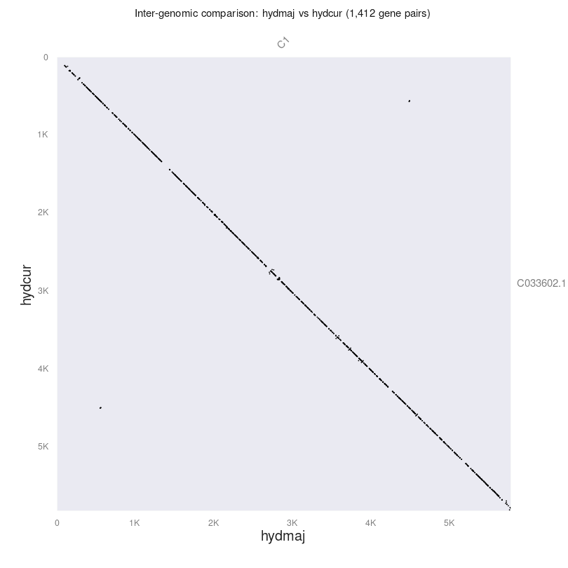
Each dot in the figure represents genes that are shared between the two samples. For the most part, these sequences are highly similar (the diagonal is straight down from top left to bottom right). There are some small regions where there are no dots at all, indicating variation between the two sequences. Further, there are some slight off-diagonal dots, indicating inverted sequences or duplicated genes.

Types of orthologs

In addition to visualising the dotplots, it may also be interesting to know what kinds of orthologs our figures are being made from. We can check this using the following command.

python3 -m jcvi.compara.synteny depth --histogram hydmaj.hydcur.anchors

This command will produce a histogram file showing the multiplicity of genes between the two sequences. Ideally, all genes would be in the 1 column, however it’s not to be unexpected that some genes are missing or have undergone duplications. This is especially true for this test dataset, as the annotation has been lifted-over from a totally different species.

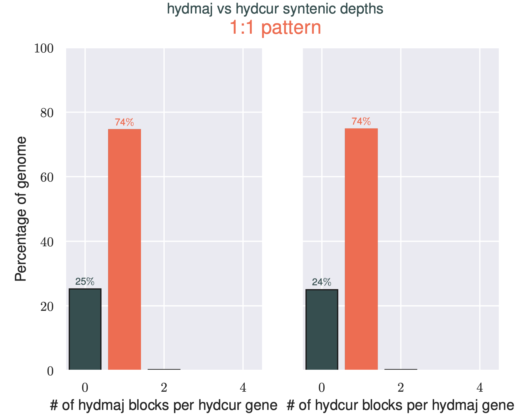
In this example, 74% of the genes in each chromosome appear only one time in the other organism, with around a quater of each snakes genes missing from the other.

Macrosynteny: Ribbon plots

To generate the ribbon plots, we’ll need to create a couple of extra files. The first is a simple seqids file. This is literally a two-line file with the chromosome name of H. major and H. curtus on each line. Normally, if you had many chromosomes, you’d order them here in this file. The seqid file for the data in this tutorial is shown below.

chr1
CM033602.1

Next, we need to create a layout file, which tells the program where to draw what. If you want to know what all the fields mean, check out the documentation. The layout file should look like the following.

# y, xstart, xend, rotation, color, label, va,  bed
 .6,     .1,    .8,       0,      , H. major, top, hydmaj.bed
 .4,     .1,    .8,       0,      , H. curtus, top, hydcur.bed
# edges
e, 0, 1, hydmaj.hydcur.anchors.simple

You’ll notice that there is the file hydmaj.hydcur.anchors.simple which doesn’t exist yet. To create this we need to run the following command.

python3 -m jcvi.compara.synteny screen --minspan=30 --simple hydmaj.hydcur.anchors hydmaj.hydcur.anchors.new 

This creates a subset of the hydmaj.hydcur.anchors file, a more sussinct form of the anchors file for plotting.

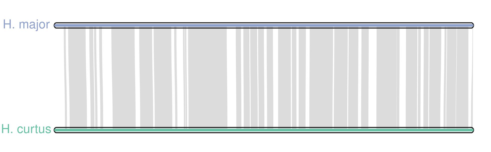
With all that done, we can now produce the ribbon plot by running this command.

python3 -m jcvi.graphics.karyotype --basepair --format=png seqids layout

The argument --basepair uses the sequence length to scale the chromosomes, rather than the synteny chunks. The final output will be karyotype.png showing the synteny between the two chromosomes.

What next?

I’ve only scratched the surface of what you can do with these kinds of figures. I highly recommend checking out the MCscan documentation to see how you can take the figures further. For more granular synteny comparisons, I recommend checking out Syri, another structural rearrangement tool. I’ve not used it before, but I’ll try and write a tutorial for it once I’ve had a go.